3D parametric field history ROM example

This example shows how to use PyTwin to load and evaluate a twin model built upon a parametric field history ROM. Such ROM, created with Static ROM Builder, has parameters that can be changed from one evaluation to another, and will output field predictions over a time grid. The example shows how to evaluate and post process the results at different time points.

# sphinx_gallery_thumbnail_path = '_static/TBROM_pfieldhistory_t250.png'

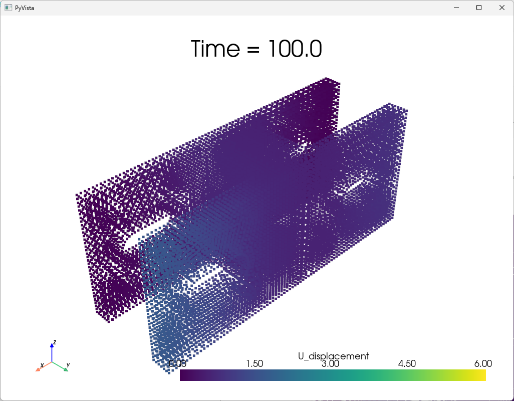
The example model is a simplified 3D mechanical frame tightened by two bolts. The bolts are represented as forces applied to the tips of the component. The magnitude of the deformation is dependent on the magnitude of both force parameters. Additionally, this component is made of a material that exhibits time-dependent behavior, allowing the structure to undergo a mechanical phenomenon known as creep. Essentially, the deformation of the structure changes over time, even under constant applied forces, which makes the problem suitable for parametric field history ROM.

Note

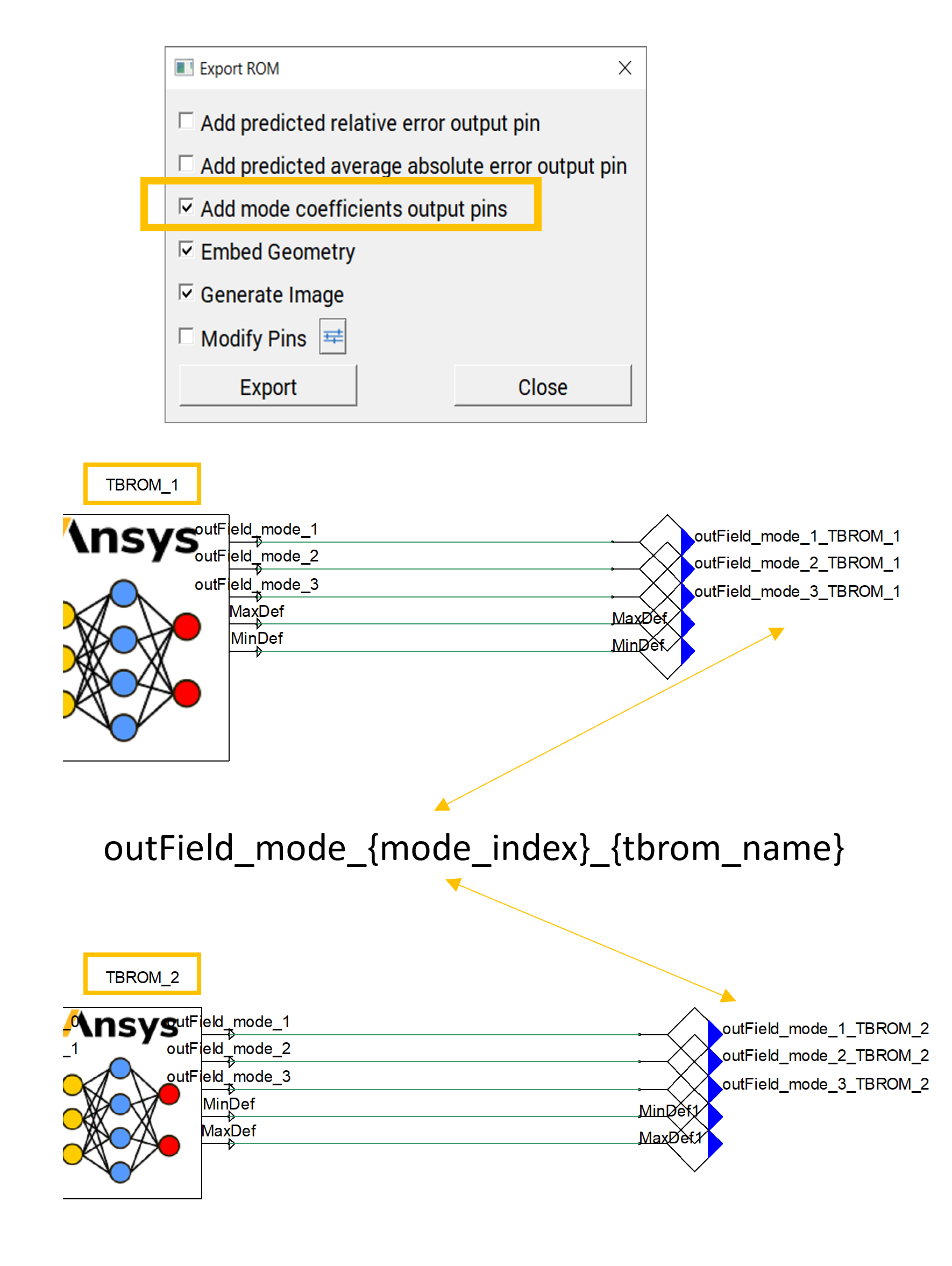
To be able to use the functionalities illustrated in this example, you must have a twin with one or more TBROMs. The output mode coefficients for the TBROMs must be enabled when exporting the TBROMs and connected to twin outputs following these conventions:

• If there are multiple TBROMs in the twin, the format for the name of the twin output must be outField_mode_{mode_index}_{tbrom_name}.

• If there is a single TBROM in the twin, the format for the name of the twin output must be outField_mode_{mode_index}.

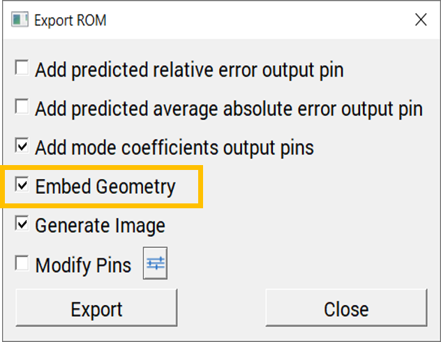
Note

To be able to use the functionalities to visualize the results, you need to have a Twin with 1 or more TBROM, for which its geometry is embedded when exporting the TBROMs to Twin Builder

Perform required imports

Perform required imports, which include downloading and importing the input files.

import matplotlib.pyplot as plt
import numpy as np
from pytwin import TwinModel, download_file
import pyvista as pv

twin_file = download_file("TwinPFieldHistory_wGeo_25R2.twin", "twin_files", force_download=True)

Define ROM scalar inputs

Define the ROM scalar inputs.

rom_inputs = {"testROM_25r2_1_force_1_Magnitude": 9500, "testROM_25r2_1_force_2_Magnitude": 16500}

Load the twin runtime and generate displacement results

Load the twin runtime, initialize the evaluation and display displacement results from the TBROM.

print("Loading model: {}".format(twin_file))
twin_model = TwinModel(twin_file)
twin_model.print_model_info()
romname = twin_model.tbrom_names[0]
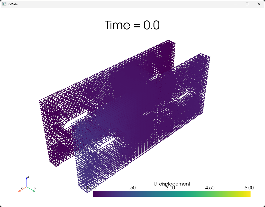
twin_model.initialize_evaluation(parameters=rom_inputs)
field_data = twin_model.get_tbrom_output_field(romname)
plotter = pv.Plotter()
plotter.set_background("white")
plotter.add_axes()
plotter.add_mesh(field_data, scalar_bar_args={"color": "black"}, clim=[0.0, 6.0])
plotter.add_title("Time = {}".format(twin_model.evaluation_time))
plotter.show()
print(max(field_data.active_scalars))

Loading model: C:\Users\ansys\AppData\Local\Temp\TwinExamples\twin_files\TwinPFieldHistory_wGeo_25R2.twin
------------------------------------- Model Info -------------------------------------
Twin Runtime Version: 2.15.0.0
Model Name: TwinPFieldHist_wGeo
Number of outputs: 5
Number of Inputs: 0
Number of parameters: 5
Default time end: 0.04
Default step size: 0.001
Default tolerance(Integration Accuracy): 0.0001

Output names:
              Name                     Unit  Type Start   Min   Max              Description
0  outField_mode_1  TWIN_VARPROP_NOTDEFINED  Real  None  None  None  TWIN_VARPROP_NOTDEFINED
1  outField_mode_2  TWIN_VARPROP_NOTDEFINED  Real  None  None  None  TWIN_VARPROP_NOTDEFINED
2  outField_mode_3  TWIN_VARPROP_NOTDEFINED  Real  None  None  None  TWIN_VARPROP_NOTDEFINED
3  outField_mode_4  TWIN_VARPROP_NOTDEFINED  Real  None  None  None  TWIN_VARPROP_NOTDEFINED
4  outField_mode_5  TWIN_VARPROP_NOTDEFINED  Real  None  None  None  TWIN_VARPROP_NOTDEFINED


Input names:
Empty DataFrame
Columns: [Name, Unit, Type, Start, Min, Max, Description]
Index: []


Parameter names:
                               Name                        Unit         Type               Start     Min      Max                                 Description
0                     solver.method  TWIN_VARPROP_NOTAPPLICABLE  Enumeration      1.000000000000     1.0      2.0  Solver integration method (ADAMS=1, BDF=2)
1                     solver.abstol     TWIN_VARPROP_NOTDEFINED         Real      0.000000000001     NaN      NaN                   Solver absolute tolerance
2                     solver.reltol     TWIN_VARPROP_NOTDEFINED         Real      0.000100000000     NaN      NaN                   Solver relative tolerance
3  testROM_25r2_1_force_1_Magnitude     TWIN_VARPROP_NOTDEFINED         Real   9500.000000000000 -6000.0  25000.0                           force_1_Magnitude
4  testROM_25r2_1_force_2_Magnitude     TWIN_VARPROP_NOTDEFINED         Real  16500.000000000000  3000.0  30000.0                           force_2_Magnitude


TBROMs information:
TBROM instance name : testROM_25r2_1
TBROM model name : testROM_25r2
Output field name : U_displacement
Output field connected : True
Has geometry/points file : True
Has input fields : False
Parametric Field History : True
Named selections : []
Product version to generate TBROM :  SVDTools 2025 R2 built on May 15 2025 @ 14:24:34

0.8973744667566538

Evaluate the twin at different time points (3D field visualization)

Because the twin is based on a parametric field history ROM, the entire field history has been computed during the Twin initialization. In order to visualize the results at different time points, the Twin can be advanced and simulated over time. A linear interpolation is performed in case the time selected is between two time steps of the field history.

# After 100 seconds
twin_model.evaluate_step_by_step(100.0)

field_data = twin_model.get_tbrom_output_field(romname)
plotter = pv.Plotter()
plotter.set_background("white")
plotter.add_axes()
plotter.add_mesh(field_data, scalar_bar_args={"color": "black"}, clim=[0.0, 6.0])
plotter.add_title("Time = {}".format(twin_model.evaluation_time))
plotter.show()
print(max(field_data.active_scalars))

1.685669230751107

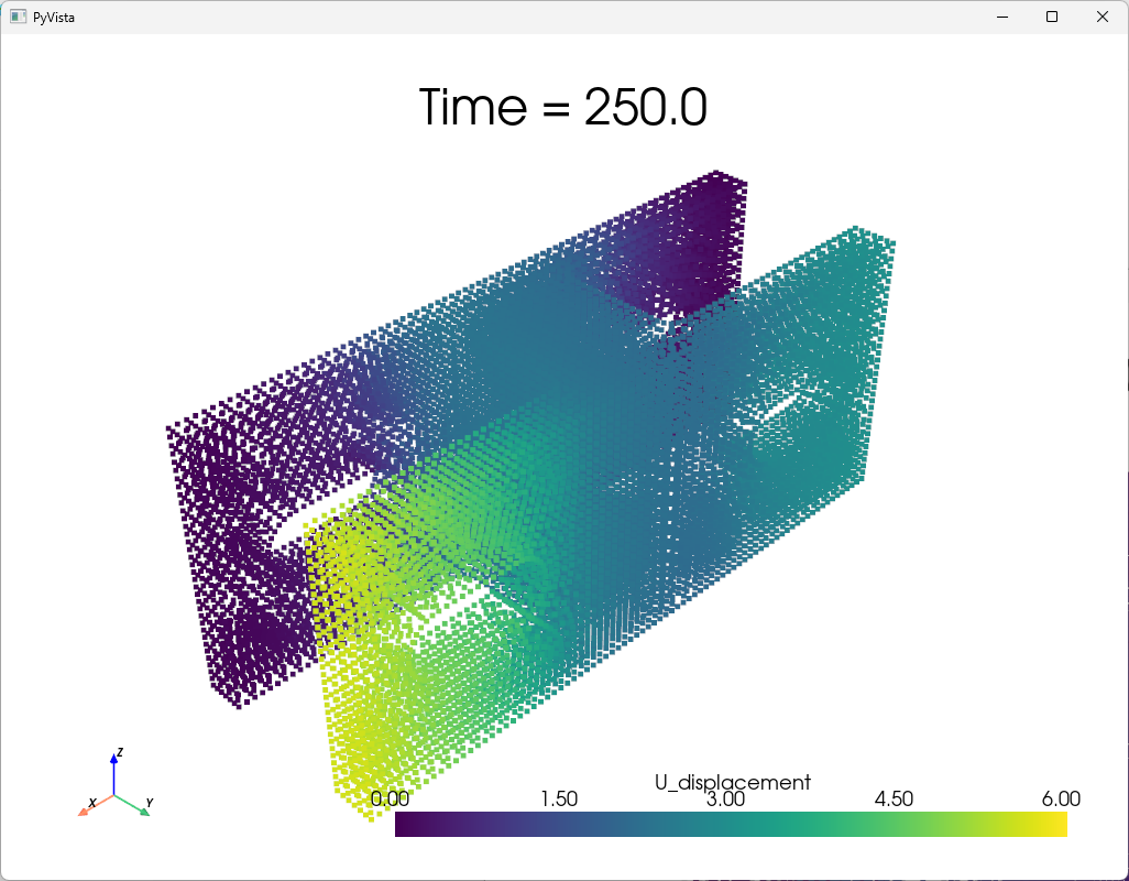
# After 250 seconds
twin_model.evaluate_step_by_step(150.0)

field_data = twin_model.get_tbrom_output_field(romname)
plotter = pv.Plotter()
plotter.set_background("white")
plotter.add_axes()
plotter.add_mesh(field_data, scalar_bar_args={"color": "black"}, clim=[0.0, 6.0])
plotter.add_title("Time = {}".format(twin_model.evaluation_time))
plotter.show()
print(max(field_data.active_scalars))

5.635884051349383

Evaluate the twin at different time points (time series)

If we continue simulating the Twin over time, the field results won’t change anymore since we have reached the end time of the field history. To evaluate the ROM again, it needs to be re-initialized, with the possibility to change input parameters values. In this section, we will see how to build and visualize a transient prediction at a given location.

timegrid = twin_model.get_tbrom_time_grid(romname)
print(timegrid)

fieldName = twin_model.get_field_output_name(romname) + "-normed"

point = np.array([0.0, 0.0, 0.0])
idx = field_data.find_closest_point(point)
outputValues = []

closest_pt = field_data.points[idx]
print(closest_pt)

twin_model.initialize_evaluation(parameters=rom_inputs)
outputValues.append(field_data.point_data[fieldName][idx])

for i in range(1, len(timegrid)):
    step = timegrid[i] - timegrid[i - 1]
    twin_model.evaluate_step_by_step(step)
    outputValues.append(field_data.point_data[fieldName][idx])

plt.plot(timegrid, outputValues)
plt.title("Displacement vs Time for point {}".format(np.round(closest_pt, 3)))
plt.show()

[0.0, 2.00000099, 9.12500096, 31.78125091, 61.78125091, 91.78125091, 120.3635355, 142.480949, 160.55882932, 176.11231065, 189.71636929, 201.93378105, 213.22661155, 223.71653536, 233.52522703, 242.67983024, 250.0]
[0.00000000e+00 3.50599992e-05 0.00000000e+00]